Stochasm

The Builder

Press Next in the Launcher and the Builder arrives. For the two designable models (Multi-Component Lattice and Patchy Discs) it comes in two steps, one card each. Step 1: structure holds the System seed knobs (lattice size or disc count and packing, and, in ensemble mode, the number of systems) and the model’s structure editors: site types for the lattice model; patch types, bead types and molecules for Patchy Discs. Step 2: rules holds the Rules editor (how the species transform, bond, and interact) and the shared Compute card (engine, workers, cell lists). The action button reads Next on Step 1 and Initialize on Step 2, where a Back button returns to Step 1: the species card dissolves into the background as the rules card flows in from the right, and Back plays the same motion in reverse. (The simpler models fit on a single Builder card and initialize directly.) Every edit re-seeds the live preview on the stage, so you always see exactly what will launch. Press Initialize and the previewed system becomes the running one; its structure is then fixed, and the header’s Back to Builder returns you here, landing on Step 2, while the run is held, paused and untouched: Resume Simulation returns to it exactly as you left it, and Re-Initialize acts like Reset Simulation, re-seeding every system from the current design (ensembles also reset their learning) while your controls, views, and windows stay put. Rules and dynamics edits made while a run is held ride along with Resume (rules apply live; the box itself never re-seeds for them). Going Back to Step 1 with a run held discards it: Step 1 re-opens exactly as a first entry, with a fresh preview and a plain Initialize on Step 2; the amber note above the Back button says so before you commit. The seed knobs and the setup flow are covered in Setting up → The Builder.

Multi-Component Lattice

The lattice model’s structure is its site types (the palette) and its rules: how those sites transform, move, and interact. Both are edited here in the Builder and shown read-only while a system runs (colours stay live everywhere; they’re display, not physics).

Site types

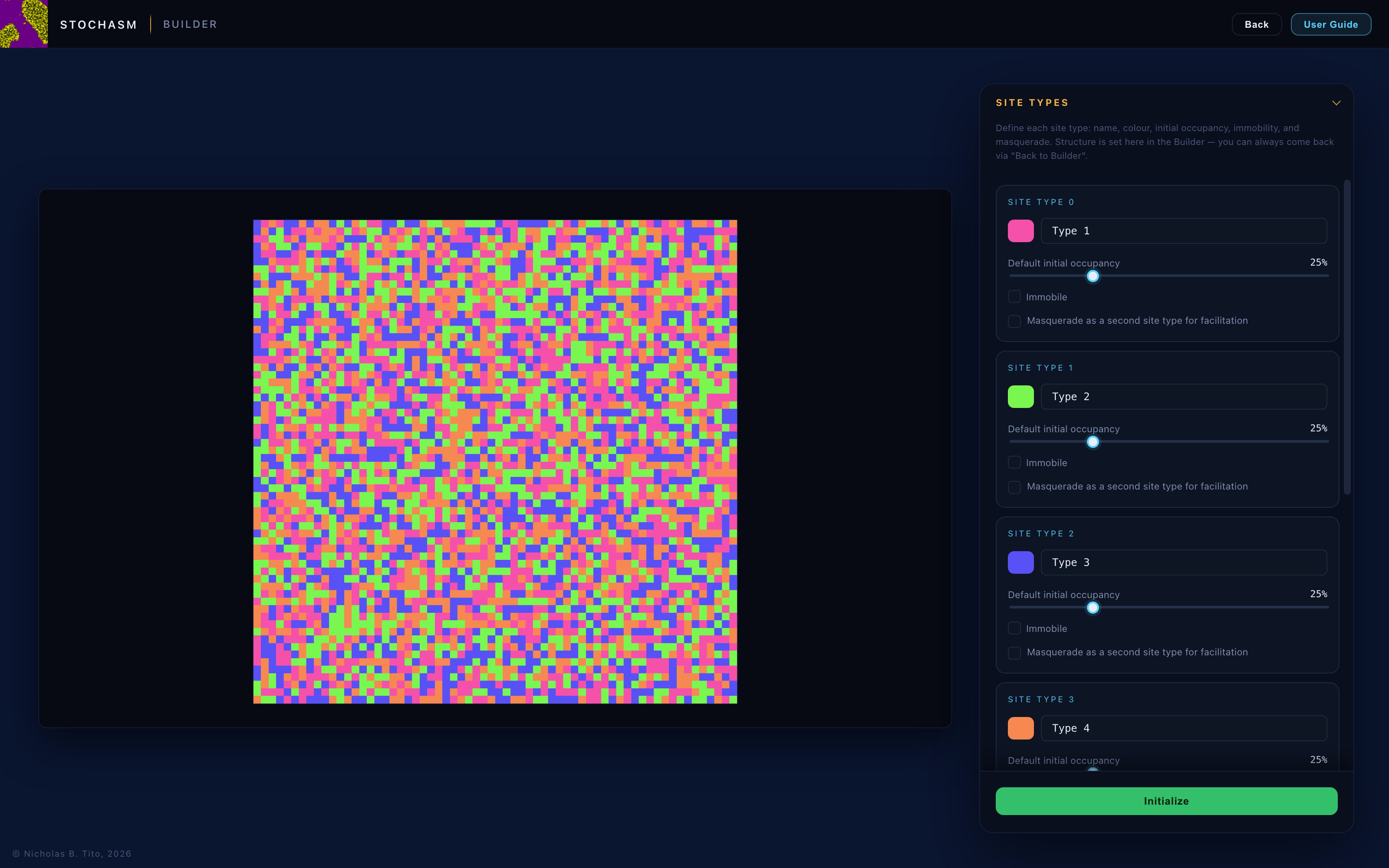
Sites are the coloured squares your lattice is made of. You can have up to ten types per system, and a minimum of two. The type count itself is a Builder decision: add or remove types here (removing one re-indexes the rules and repaints its sites), then Initialize. Each type carries:

Rules

Rules are the verbs of your system. There are four kinds, each with its own glyph (drawn between the two endpoint swatches) and matrix code:

A rule’s structure (its name, kind, and two endpoints) is fixed here in the Builder (endpoints and kind can’t change once created; delete and re-create to change them). Each rule names a specific type on each end, or the any-site wildcard. Its parameter, the raw attempt-weight for flips and swaps (0–1) or the interaction energy for a Site-Site rule (−10 to +10 k_BT, negative = attraction), is tuned live once the system runs, under Simulation → Rule Controls. A newly-created flip or swap starts at parameter 1 (full attempt rate); a new Site-Site Interaction starts at 0, energetically neutral until you dial it in.

Facilitation. A flip rule can be made conditional on the neighbourhood: set Requires Neighbour Site to some type and a # of Neighbours Required (1–8), and the flip only fires at sites with at least that many neighbours of that type. This is the ingredient of kinetically-constrained models: the FA preset is exactly one facilitated flip. Masquerading types count toward the requirement of the type they imitate.

The interaction matrix. The Builder shows a type-by-type matrix of your Site-Site Interactions and facilitation gates as symbolic dots; once running, the same matrix under Simulation carries the live SS energies and f(●)×n facilitation chips. If two enabled SS rules address the same pair, the later one wins and the matrix flags the duplication with an amber warning.

2D Ising

The Ising model has no palette to build: every site is one of two spins. Its Builder is minimal: the lattice size and, in ensemble mode, the number of systems, plus a starting condition (hot, cold, or aligned up/down) chosen in the Launcher. Everything that shapes its behaviour (temperature, coupling, field) is a live control in the Simulation stage.

Single Particle

The single particle’s “structure” is the potential it lives in. You choose a single well (a harmonic trap set by its frequency) or a double well (set by a separation/depth and a left/right bias); the Builder itself only sets the ensemble size. The potential shape and the rest of the Langevin dynamics (temperature and friction) are tuned in the Simulation stage.

Patchy Discs & Polymers

Patchy Discs & Polymers is the off-lattice member of the family. Its design splits cleanly in two: bead types are the palette — what a bead is (size, shape, colour, patches) — and molecules are the population — what actually stands in the box: free discs, or bead-spring chains. Around them sit patch types (the coloured triangles riding on disc rims; each triangle’s tip points along its bonding direction) and rules: either patch–patch bonds or disc–disc attractions.

Designing particles

The Particle design editor stacks three cards. Patch types are the bonding species: a name and a colour, drawn as triangles everywhere they appear. Below them, each bead type carries a name, colour, radius, two shape-distribution knobs, and its list of patches, each one a patch type placed at a rim angle in degrees. A bead type carries no count: it says what a bead is, never how many there are. The shape knobs make a species irregular: Smoothness below 1 gives every particle its own unique bumpy boundary, drawn at initialization from a low-mode random spectrum (the lower the smoothness, the stronger the bumps), and Polydispersity spreads the base radii (a clamped Gaussian of that relative width). Each particle in the population is one-of-a-kind. Physically, an irregular pair repels (and, under a disc–disc rule, attracts) through the usual soft potential evaluated with the local contact distance: the sum of the two surface radii along the line joining the centres, so the shape genuinely pushes, twists (bumpy contacts exert torque), and packs like it looks. Patches ride the true local surface at their angle, so bond anchors and bonding geometry follow each particle's own boundary. Add and remove freely; every edit re-seeds the box preview live, so it always shows what will launch. Patches are optional: strip them all (and even remove every patch type) for bare discs that interact only through their soft core plus any disc–disc attractions; the patch-bond matrix and the patch–patch rule kind simply disappear when no disc carries a patch.

The Molecules card underneath is the population. Each molecule names an architecture — Single disc, Homopolymer, or one of the copolymer sequences described below — picks the bead type it is made of (two of them for a copolymer; a custom sequence names its own), and sets an abundance, its share of the discs in the box (the readouts show the normalised percentages). A chain molecule adds Beads per chain and Bead-count spread, plus whatever its architecture needs. The same bead type can appear in several molecules — free monomers and chains of the one species — and a bead type used by no molecule simply never appears in the box. The readout in the System card, just below Regenerate initial configuration, counts what the current draw actually produced. During a run the design is read-only (colours stay tunable, display only); to change anything structural, press Back to Builder.

Bead-spring polymers

A polymer is a molecule with a chain architecture: a linear chain of Beads per chain beads — and every bead is still the bead type you designed, carrying its radius, colour, roughness, polydispersity, patches and disc–disc rules. So a polymer with patches can crosslink into a network, and one with a disc–disc attraction collapses in poor solvent; nothing about the rest of the model has to change.

A Homopolymer is all one bead type. The four two-component architectures mix two bead types (pick both in the card) along one backbone: a Diblock is an A-block then a B-block, split by the Block fraction slider; a Multiblock alternates A- and B-blocks of Beads per block each (1 makes the strictly alternating copolymer); a Gradient runs linearly from pure A at the head to pure B at the tail, each bead drawing its type from the local composition; and Random draws every bead independently at the Composition you set. The molecule’s dot icon previews the pattern. Sequences are drawn when the box is built — regenerate for a new realization of the random ones.

Custom sequence is the general case: you write the chain out bead by bead. Each bead type gets a letter by its position in the palette — A is the first bead type, B the second — and a number after a letter repeats it, so A6B12A6 is a 24-bead ABA triblock and ABAB a four-bead alternating one. The card shows a legend of which letter is which, and underneath, the chain itself as a row of beads: click any bead to change its type. Typing and clicking edit the same thing, so use whichever suits — the field for long regular patterns, the beads for touching up a few. The sequence fixes the length exactly, so a custom chain has no bead count or spread of its own. This is how you build architectures the other five cannot express: a triblock, a tapered end, a sticky cap on one side only.

One honesty note for chains that mix bead sizes: the crossing-free seeding lattice is spaced for the largest bead type, so a population dominated by much smaller beads can need more lattice sites than the packing-fraction-derived box provides. Stochasm then enlarges the box until everything fits: chain lengths and abundance stay exactly as designed, and the packing fraction comes in under the slider — the System readout shows the real box.

Bead-count spread is a polydispersity in the length: 0 makes every chain the same, higher values draw each molecule’s bead count from a Gaussian around your setting — real polymer samples are never monodisperse. The readout in the System card (below Regenerate) tells you the thing you actually want to know: how many chains your disc budget currently buys.

The length distribution is sacred. The box fills with whole molecules and stops at the first one that will not fit — a chain is never trimmed or shortened to squeeze the disc count to an exact number. So at spread 0 every chain really is your bead count, and at higher spreads the realised lengths are genuine draws from the Gaussian you asked for. The cost is small and honest: the realised disc count can land a shade under the slider (by less than one molecule; the readout says so), while the packing fraction stays exact because the box is sized from what was actually drawn. At extreme packing fractions (φ above roughly 0.65) the seeding lattice runs out of room and whole molecules may be left out rather than cut down — the box simply comes in a little emptier.

The chain’s angular stiffness κ is not here, because it is dynamics rather than structure: like a rule’s ε, you tune it live while the system runs, under Simulation → Chain Controls. Bending does not affect how the box is built, so changing it never re-seeds anything.

The bond itself is the same harmonic spring a patch bond uses — same global bond stiffness slider — pulling neighbouring beads to touching distance. It acts on the bead centres, so it applies no torque: κ alone decides how floppy a chain is.

Chains never start crossed. This matters more in two dimensions than you might expect: flat chains cannot pass through one another, so any crossing present in the starting configuration is stuck there for the entire run — no amount of simulation will untangle it. Stochasm therefore builds the initial box by threading each molecule through a hexagonal grid of sites, one bead per site, never revisiting a site it has already used. Grid edges cannot intersect and no two beads share a site, so the box begins with zero crossings and zero overlaps by construction, at every packing fraction, with the bonds already sitting at their natural length. The chains look a little orderly for the first instant; the thermal velocities scramble that within a few steps, and the topology you get is one the dynamics can honestly preserve.

Abundance still means the share of discs, exactly as it does for a single-disc molecule — set a chain to 75% and roughly three in four discs in the box belong to chains, however long they are. What changes is the molecule count: the box is filled with whole chains up to the disc count you asked for, so 100 discs of 24-bead chains is four molecules, not 100. Raise the disc count for a real melt, and expect the split to sit closer to the slider the more discs you give it. Under Compute a Polymer chains observable group appears, measuring each chain’s radius of gyration and end-to-end distance — the two numbers that say whether your chains are coiled, swollen, or stretched.

Interaction rules

Every rule has a kind, chosen when you create it. A Patch–Patch rule makes one pair of patch types bindable: a directional Kern–Frenkel bond, formed and broken by Monte Carlo. A Disc–Disc rule adds an isotropic Lennard-Jones attraction between two disc species: a soft well of tunable depth that the molecular dynamics handles directly, no bonds involved (so it can drive condensation and demixing). Both live in the same list, tagged BOND or LJ; with no rules at all, discs feel only their hard core.

Rule structure (a name, the kind, and the two endpoints: patch types for a bond, species for an attraction) is fixed at creation, so delete and re-create to change it. The dynamics are tuned live under Simulation: the strength ε (bond well depth, or LJ well depth) for either kind, plus the bind/unbind attempt rate for patch–patch bonds only. Toggle a rule off there to remove its interaction mid-run. Two matrices summarise it all (a patch-bond matrix and a separate disc–disc matrix): symbolic dots here in the Builder, live ε values under Simulation; only the lower triangle is shown, since both interactions are symmetric. Each matrix appears only when it has something to say: the patch-bond matrix hides for bare-disc designs, and the disc–disc matrix hides until the first Disc–Disc rule exists.